Hello there!
It’s 4/20 and I hadn’t written a blog post in a little while. Instead of the devil’s lettuce I thought, “what better activity could we do?” So let’s clean off the spider webs and crack open our physics textbooks. We’re going to derive the Einstein field equations! I assure you, they’re a hoot and a half! Or at the very least you’ll see a lot of corny Pythagoras jokes, and that’s just as important.
Readers should know that general relativity is something you’d only really understand after taking a graduate course in physics. This blog post is not a substitute for that course. But this post does show you a lot of the concepts that were relevant for deriving the theory. The majority of the derivations here were originally published and refined by Einstein between the years 1905 and 1915. Don’t worry about the math, what’s much more interesting here (for me anyway) is the concepts and how they came about.
- Introduction
- The Field Equations
- Metric Tensor
- The Christoffel Symbols
- Curvature
- Stress Energy Momentum Tensor
- The Cosmological Constant
- Putting the pieces together
Introduction
History
Part of the appeal of learning these equations is the fleeting feeling that perhaps you’re on the same intellectual footing as one of the greats such as einstein. Einstein has always had a perception of being one of the greatest physicists of all time. I think that this perception is a little bit unfair to the other scientists who were doing incredible work at the time.
I want to start this post with some background on einstein that I found in a very insightful comment on reddit. Here’s a portion of that comment on how einstein came to be seen as synonymous with intelligence.
In the early 20th century, there were a handful of scientific heroes. Many of them have not persisted in /public imagination. Almost nobody outside of the sciences today is going to know who Robert Millikan is, but for a time he was the most famous scientist in the United States, for example.
Einstein’s international fame was the result of several distinct events that led him to be branded as “revolutionary” on a level above and beyond his peers (and perhaps above and beyond his accomplishments).
In 1905, when Einstein published his first papers on relativity theory, he was virtually an unknown. For the next decade, he became a little better known in the community of physicists, but even then practically nobody worked on relativity without having a direct personal connection to Einstein in some way. If you look back on those papers with a sober eye today, they are interesting, and the fact that all four of them came out in the same year is rather impressive, but they are not heads-and-tails more revolutionary than other work being done at the time. The paper on the photoelectric effect (for which Einstein got the Nobel Prize in 1921) is important in that it shows that Planck’s idea of the quanta has physical meaning (and is not just a mathematical heuristic, as Planck thought it was), the paper on Brownian motion is an interesting (if not strictly necessary by that time) way to argue for the physical reality of atoms. The paper is an interesting derivation but it was not at all clear it had any physical reality (and nobody, including Einstein, thought it had any practical applications). The length contraction/time dilation (special relativity) paper is an interesting approach to a curious physical puzzle (what happens if you take Galilean relativity seriously, but believe the speed of light is invariant?), but again, doesn’t really get you anything obvious out of the physics, and it wasn’t clear if it was physically real or not. In short, these papers did not shake the world up, but a few people took note.
Awareness of Einstein perked up a bit in the 1910s, as he was one of the only German professors to protest against World War I (both the English and German professoriate were largely belligerent and issued long “manifestos” in the name of their countries). In 1915 he published his theory of General Relativity which was much more mathematically complex than his previous work, and much more ambitious in terms of its implications. Here was a new theory of gravity, in the end, one that would explain anomalies with Newton’s theory of gravity, but also would explain what gravity was in a way that Newton could not. This would be of much more interest to astronomers, if it were true.
Ironically, perhaps, the place where the most latent interest for General Relativity would exist was the United Kingdom, in no small part because the mathematical training required as part of the British tripos system made the British scientists on the whole much more competent at such matters than those scientists on the continent (the German tradition of physics was more strongly rooted in experimental procedure, and the math of General Relativity is of a high-enough order that your average German experimental physicist of that time was not really capable or interested in dealing with it). One British astronomer/physicist, Arthur Eddington, decided in the postwar period that it would be a really splendid thing to see if Einstein’s theory was correct. Eddington had more than scientific motivations: he was a British Quaker, and he thought it would be an impressive demonstration of the unifying powers of science if, in the wake of the Great War, he were to undertake an expedition to prove correct the theory of a German Jew. What could be more international and pacifistic than that?
So Eddington put together an expedition to the island of Principe to take photographs of stars near the edge of the Sun during the total solar eclipse of 1919, which, if combined with photographs of the same stars when seen from that position at a time when the Sun was not in the sky, would allow one to see if the starlight had been bent by the gravitational field near the Sun (a prediction of General Relativity). Eddington found that this was so and undertook to /publicize this discovery widely — Newton had been overturned.
This received national newspaper coverage worldwide. Now Einstein started being known as the guy who overturned Newton. He quickly became an international celebrity, and he capitalized on this by traveling much, giving lots of lectures (which also conveniently got him outside of Germany, where anti-Einstein and anti-Semitic forces were mobilizing), and writing at length on lots of topics. Because Einstein was not just interested in science. He wrote at length about philosophy, politics, socialism, pacifism… he made a name for himself not just as a scientist but as a /public intellectual.
Which, it should be said, still might not have cemented his long legacy. Other scientists did such things. It is not at all clear that Einstein was truly the most intelligent man of his time. He had a lot of competition — there were a lot of smart people around then, including people whose contributions to physics were no less enduring. There were also other /public intellectual scientists of the time, many of whom have been forgotten to all but science historians. Einstein’s physics is clever, but it is less “out of the blue” than it looks if you look at it in its context than in isolation. (Typically when Einstein’s work is taught, it is taught in juxtaposition to people like Newton, not in juxtaposition to the science of his time, which is largely forgotten. If you put Einstein’s work up next to, say, Lorentz and Poincaré, it looks more “of a piece” with what was being done at the time, and his early work looks relatively crude. This does not diminish it, but it is a lesson about the difficulty of properly assessing a scientist without looking at their actual context.)
With that background in mind, Einstein’s work is some of the most important physics that’s happened in quite a long time.
This post is going to discuss a lot of the mechanics underneath Einstein’s theory of general relativity, and hopefully give you an understanding of how it came to be.
Math
So let’s start with some basic assumptions that i’m making about you, the reader.
You should know some calculus and a little bit of linear algebra. It’s gonna come up unfortunately.
Equivalence
If you’re in a room with no windows, you can’t tell the difference between being in a box that’s accelerating through space accelerating at , and a box that’s on the earth while experiencing the same force of gravity . That’s essentially the equivalence principle.
Now on earth specifically the value of g varies due to tidal forces but that’s not really the point here.
Curvature of light
You’ll also need to know that light bends when traveling through a gravitational field. Let’s be more specific.
Imagine you’re traveling in a windowless room that’s accelerating upward at the speed . If you shoot a laser horizontally across the room you would expect it to land at the same height on the other side of the room. Now of course light travels forward and if the windowless room is accelerating we observe something different. As time moves forward and the room moves upwards, the landing height will become lower and lower by the time the light reaches the other end.
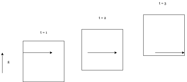
The first of what is sure to be many diagrams in this blog post.
So the light was pointed horizontally forward, but when it reached the other end of the elevator the light was lower on the other side of the room. The light curved. Because the equivalence principle tells us that we can’t tell the difference between this situation and the situation of the stationary situation on earth when influenced by gravity that results in an interesting conclusion that must be the case.
That the light must be curved by gravity in order to be true.
It turned out to be proven during a solar eclipse (that story about Eddington from the history section) when they were able to see a star that appeared to the right of the sun, despite astronomers knowing for a fact that the star was behind the sun. This meant that the light from that star was being bent around the sun.
Newton’s laws of gravitation gave us a simple way to look at gravitation at that time.
note: here is the gravitational constant, and are the masses of the two objects, and is the distance between them.
But light has no mass… why is it being affected?
This was the central problem, and the whole point of why this was a huge deal.
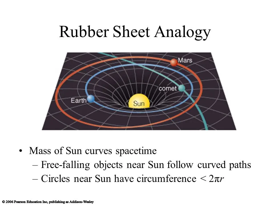
Einstein says to imagine that spacetime is like a trampoline. When you stand on a trampoline you’ll notice that the space in the trampoline indents around you in response to your weight as you sink in.
Apparently standing on a trampoline is the best allegory for spacetime that physicists could come up with.
If you put a marble near you and stand on the trampoline, you’ll notice that the marble rolls towards you.
Newton believed that this was because of the gravitation between the two objects.
Einstein believed that this was the marble moving along the shortest path in curved spacetime.
He went on to argue that the same thing was happening on the planetary scale as well. That the earth is rolling along what is really a straight line in curved spacetime around the “disturbance” caused by the mass of the sun.
note: when we say spacetime here, what we’re referring to is 3 dimensional space coupled with time.
also space and time are “the same thing”. (It’s more honest to say they’re intertwined, but physicists aren’t honest.)
Here’s why:
It started when Einstein showed that some basic laws of the universe affect both space and time equally. For example when a train is moving really fast a strange thing happens:
People who are watching the train see that the time for the train and people inside it slows down. People inside the train see that the distance in front of them is getting shorter.
These observations are not in contradiction, both groups (the observers and the people inside the train) are equally right even though one of them is seeing the time is affected and the other one is seeing that the space is affected. So we say that spacetime is affected.
Yes, time is slowed down for those on the train. That is what Einstein discovered. The faster the object is moving the slower its time seems for those who are observing it. It is called special relativity. This only becomes significant if the object is moving extremely fast, close to the speed of light. There is also general relativity which says that also gravity affects time, stronger gravity will slow down time more.
Note that the people inside the train will perceive their own time normally, it will only seem slower to the people outside the train. It is also interesting that the poeple inside the train will see that the time is slower (not faster!) for those outside the train. This leads to so called twin paradox and is actually hard to grasp at the beginning, you may need to read something on special relativity.
The Field Equations
This is the formula communly known as the “Einstein field equations”.
Here, and can be any of the 4 dimensions (values 0 through 3). (accounting for the 3 dimensions and time) Every single parameter can be substituted in any way and the equation will still be true. In this sense it’s more like 16 equations. There are a few duplicates so they reduce to about 10 equations.
The other constants are ones you’ve seen before:
- is pi.
- is the gravitational constant
- is the speed of light.
- is the cosmological constant.
- is the metric tensor.
- is the Ricci curvature tensor.
- is the curvature scalar.
- is the stress energy momentum tensor.
you know it’s an important equation when it contains the cool stuff like and .
So the whole point of this equation is that it balances two things:
- The left side refers to curvature of spacetime
- The right side is about mass and energy.
These equations show us that mass tells spacetime how to curve and that curved spacetime tells mass how to move.
if this information is satisfactory for you then you can stop reading now, the rest of the post is all math, and who wants that?
Metric Tensor
Imagine you are a person standing on a grassy field with lots of hills and you wanted to model your height above sea level as a function of where you moved.
So you start at your original position in this field from fixed point (, ). And let’s represent our height as .
Now when you walk straight through a field with hills you’ll walk up some hills and down others which of course is a change in height. So to represent our height as a function of which direction we walk in, we will use the following equations for the and directions.
These two equations essentially say that the change in height () can be derived by multiplying the rate of change in that direction, (also known as the gradient), and the actual distance you moved.
So if you walk 5 meters down a 1/10 incline, than you’ll be 1/2 a meter lower. (shocking I know.)
becuase
So this is a quite general form. The value of our field is multiplied by the gradient, or change in field, times the distance you traveled.
Of course a 1/10 slope isn’t going to happen at your grandma’s favorite park, but it will happen at much smaller distances! (This is why we have . Which means unfortunately calculus is probably involved.)
We need to deal with one other thing. People don’t walk in boring straight lines like and . Straight lines suck!
So let’s get a little more abstract. Any path along a field is going to involve components of and . So let’s represent all possible paths as a combination of the two in a more generic equation. We’ll call our combined path .
If you’ve done literally any physics ever you know that to combine these vectors we need to talk to the hotdog choreographer himself, mac daddy pythagoras.
this will give us the magnitude (or length) of the combined vector .
Of course we can add these vectors as well.
So our representation of height as a function of movement along path looks very similar, we’re just adding the changes in height contributed by the movement along each direction.
if you needed more foreshadowing here, you can probably abstract this concept to as many dimensions as you want…
This means that we can do another substitution based on what we’ve already done earlier with the and direction and add in our definitions for and
Yes I know, we switched from to , this is just a semantic distinction to make clearer for the math people that the rate of change is specific to the variable we’re looking at in that term, but not the only rate of change we care about.
So up until now we’ve been using and . Again we could use any set of coordinates here, variables are just labels after all.
So let’s abstract further, and our equations that we’ve been building so far will use different variables.
We’ll switch with and with .
That leaves us with the convenient feature of being able to consider further terms and abstract to as many dimensions as we want. So we can go up to dimensions.
Equation 1:
That weird just means we add up all the terms based on , if is we’d get the equation above we just made. On a totally unrelated note look how awesome that math term looks. You just know we cooked up some serious bullshit right there… uh, let’s continue.
Now we’ve done a lot of math relating gradients and their effects from the reference frame of a single observer about their height as they walk through a field.
Now we know from earlier that time and space are related in strange ways that result in time dilation and length contraction. That “reality is observed differently” by observers in different reference frames.
If we’re ever going to make a statement that’s universally true, it has to be true in every possible frame of reference as well. The first thing we’d need to be able to do is model the two reference frames and relate them.
So if two people are walking through the same grassy field, how would we model all the gradients of person from the perspective of person ?
Well it turns out we can do this. Let’s say we want to model all the gradients of person : we’d use the chain rule to parse out what that looks like.
I’m going to use reference frame as an example. Meaning observing all the gradients of x from an observer in the “y_1” dimension. That hill analogy is certainly getting a little strange but bear with me.
Now you’ll notice this can also be abstracted to an arbitary number of dimensions.
Equation 2:
$$ \frac{ \partial \phi }{ \partial y_n } = \sum_m \frac{ \partial \phi }{ \partial x_m } \frac{ \partial x_m }{ \partial y_n } $$note: here we’re using as our summation variable, and using as an identifier for the dimension of our observer. We don’t have to be using here, it could be , , , ,
Tensors
So it’s about time we talked about tensors. The whole point of all of this crap has been to talk about the metric tensor yet we still haven’t gotten to it. Let’s talk about what a tensor is for a bit and then we can get to the good stuff.
Equation 3: the vector transform
We can modify our equations from earlier a little bit to develop something you could call the vector transform. Essentially meaning that the th coordinate of a vector in the frame of reference is equal to the sum of the gradient term times the th coordinate in the th frame of reference.
The idea here is essentially for a vector with coordinates we can construct a representation of a vector from the perspective of by “transforming” the vector from the x representation.
It will be helpful to start with scalars first. A scalar is a quantity with no direction associated with it, temperature is a good example of this. Contrast this with a vector which is just a scalar with a direction (like velocity).
You could think of a scalar as a tensor of rank 0. Then a vector is like a tensor of rank 1.
Now a tensor could be thought of as a combination of vectors where there is a fixed relationship between the two.
Imagine the example of a block being pushed by a force:

try to ignore that weird angle bend in the image i’m trying my best here.
So there are two forces here, and , note that only actually moves the box, and it’s moved a distance .
If you imagine that is the only force acting on the box, we know that the work done on the box will be equivalent to the force times the distance along the direction that the box moves in. Now of course there’s an and component to the force that’s acting diagonally on the box so we have to do something different here to evaluate the work done on the box in the direction and we can resolve that problem pretty quickly.
So that’s all fine. Now lets think about .
The work done by is because is . But more obviously if you push down on a block it won’t move.
This basic mechanics example has an important property. No matter what reference frame you view from, the outcome is exactly the same. The block does not move.
A tensor is the relationship between two vectors. If a tensor has a value of in one frame of reference, it has a value of in all frames of reference. The block never moves.
You might guess that this concept is going to be very useful in our discussion of Einsteins theories of relativity.
Ugh I sound like such a textbook.
Let’s bring it on home. Imagine two vectors (who cares what they are): We’ll look at the th dimension of and the dimension of . We’ll say that the combination of the two creates a tensor of rank 2.
Now there’s something important to point out here, which is that and are dimensions. In our examples so far we’ve been in the plane so and both are either or . This means there are four possible tensors to create between the two vectors.
If you have dimensions in space, then there are 9 different versions of and so on.
Now what would and look like from the reference frame of ? Let’s use our equation 3 from earlier.
So now let’s simplify that a little bit with some condensing, and we get toooooo
Equation 4: the contravariant transformation
You’ll notice that this is an equation that enables you to transform , (better known as T_x^{rs}) into T_y^{mn}. Hence it is known as the contravariant transformation. If you’d like to make this harder to understand feel free to check out wikipedia.
this is getting harder to follow along in an obvious way. I know. I’m sorry. For what it’s worth, writing this all out and formatting the math has been a nightmare.
Here’s an alternate version of equation 4 that you should know about
Equation 5: the covariant transformation
Now we’ve come a long way talking about a lot of stuff that’s not the metric tensor. Like most physics textbooks we’re going to continue that trend by taking yet another look at the justin beiber of philosphers, that’s right. The mac daddy pythagorean theorem. Like good physicists we’ll draw a fun diagram and apply what we know to arrive at something we don’t. Afterwards, again like most physics students we’ll think we understand it after reading it and then fail to reproduce it in the future.

Let’s examine this example triangle. Obviously the variable names for the lengths of the sides are completely coincidental.
We’ll start with an initial pythagorean understanding of the situation.
Now what you might have heard is that the phantom menace pythagoras wrote a theorem is actually just a specific instance of a more generalized rule. We can actually expand it out.
Then we can restate it.
Now for this to still be consistent, we have to make sure we’re not taking any products we don’t want in the sum.
And so that’s that that is for. That there is the Kronecker Delta.
The kronecker delta is a funky machine. Essentially on every iteration of the sum operation for new values of and , is evaluated to be either 0 or 1.
So if then , and otherwise .
The delta is essentially a scaling factor so we can take it out like anything else.
Now we can use our definition from before:
When we apply that to our working definition of ,
Now we’ve got something quite powerful. Let’s just rearrange this for a second.
And there it is. The beautiful metric tensor.
The metric tensor
So… what does that really mean? Like most physics courses, we’ve barely said anything about physics for about 10 minutes and spent the majority of our time doing derivations. All we have is some cool looking math to show for it!
To understand what the metric tensor is let’s look at the original sinetist (heh), pimp daddy pythagoras just one more time.
Looking back at our more generalized approach from before, take a look at what happened.
So our normal pythagorean theorem is functional for flat space. In flat space it’s perfectly true that we can use the normal pythagorean theoem.
Now imagine we have that same right triangle drawn on a sphere. We wouldn’t be in flat space anymore, if we had the same right triangle on the surface of a sphere, we still couldn’t use meme lord pythagoras. So what the metric tensor gives us, is a device that corrects for operating in curved space.
So i’m sure you can see how this is going to be valuable when operating in curved space.
So our term works in that way, and that’s what that term is when looking at the field equations.
note that the terms there are just a convention that is often used when talking about spacetime. Again, they’re just indicators for whatever dimensions you’re condidering.
The Christoffel Symbols
The important thing about tensors is that they represent a relationship between two vectors that’s true in all reference frames.
let’s imagine a tensor
Here’s the problem. One thing that will come up pretty quickly when examinig tensors is that the derivatives of tensors don’t have the same powerful fixed properties that derivatives of vectors do.
Are the derivatives of tensors the same?
If we look at the derivative of with respect to in the frame of reference, does that equal the derivative of with respect to in the frame of reference.
Does ?
Let’s look again at equation 5:
We can use that and apply it to our question substituting for .
We’re substituting it in which is why we’re using instead of .
which simplifies :
Again, what we’re trying to determine, is if is equal to .
I’ll save some time here and just show what is.
note that the still applies here. I just didn’t write it. Einstein actually believed that writing it out was trivial and that it was implied.
So upon examination it turns out they’re unfortunately not equal. They’re quite close!
If you look a little closer the only difference between the two tensors is those extra terms at the end of .
here’s those terms again just to be clear.
Those extra symbols at the end there are called the christoffel symbols, and are often abbreviated as .
So the question we asked was is if .
We found the answer is no, however we can still work with this using something called the covariant derivative.
Equation 7:
The christoffel symbols exist as a correction for the transformation of the derivative of a tensor from one reference frame to another.
So we did that for vectors, and now we’ll need to do it for tensors. So let’s look at the covariant derivative of .
Equation 8:
And there we have it! That’s the transformation of a tensor from one frame of reference to another! Swag.
So just a quick concept check, what would the covariant derivative be of in flat space?
The covariant tensor of the metric tensor in flat space is zero.
In flat space the metric tensor is either 1 or 0. Either way it’s a constant, and the derivative of any constant is zero.
Here’s how that would apply within equation 8.
P.S. If professor Schnetzer at Rutgers is somehow reading this, here’s a free exam question for you next time you teach General Relativity.
So we can rearrange this with the help of some crazy mathematicians.
Equation 9:
$$ \Gamma^a_{bc} (x) = \frac{1}{2} g^{ad} \Bigg\{ \frac{ \partial g_{dc} }{ \partial x^b } + \frac{ \partial g_{ab} }{ \partial x^c } - \frac{ \partial g_{ab} }{ \partial x^d } \Bigg\} $$Now we have our equation for the christoffel symbol in terms of first derivatives of the metric tensor.
Now if you’re wondering why we care about the christoffel symbol, it’s because it’s a part of the ricci curvature tensor which is a part of Einstein’s equation.
Curvature
We’re going to have to define some other operations before wee can go on to the ricci tensor.
Commutators.
This is a commutator operation on some sample matrices and .
Ricci Tensor
So the Ricci tensor is the part of the curvature of spacetime that determines the degree to which matter will tend to converge or diverge in time.
This may be slightly misleading, so i apologize if it sounds confusing. Vectors change due to curvature.
This change can be modeled in the following way.
You can break this down using that down that commutation definition and equation 7. I’m gonna skip it for now and leave this as an exercise for some non-lazy reader.
The ricci tensor is made of christoffel symbols and derivatives of christoffel symbols, which themselves are made of metric tensors and the derivatives of metric tensors. And metric tensors, again are simply a tool to correct for the happy slapper mac daddy pythagoras when applying his nonsense in 3d.
So the Ricci tensor is the terms in our model.
i’m skipping a few steps to save time, mostly because typing out latex to this extent is a nightmare ~
It could be called the Riemann tensor, but for the purposes of relativity we’ll say that this is the Ricci Tensor.
Curvature Scalar
I’ll save some time and say that from the ricci tensor, you can derive the curvature scalar. It’s simply a scalar, not a tensor, not a vector.
The point here is if the curvature scalar is not , then the surface is not flat.
Stress Energy Momentum Tensor
Let’s start with a quick definition.
Geodecic - the shortest line between two points that must travel along a curve. Examples are things like the equator, and any line drawn on a sphere.
So let’s imagine what it looks like if we take a tangent vector of a geodecic. We can define a tangent vector as a rate of change of the distance we travel with respect to time.
Wheat we’re interested in is to find the minimum path along a geodecic by taking the derivative and setting it equal to zero.
Now remember we have to take the covariant derivative here because 3d so we’ll use equation 7:
here is the proper time. the gamma term is larger but we’re going to move it around in a moment so i haven’t expanded it here.
We can simplify the time derivative:
It’s worth noting, that is a second derivative of distance with respect to time. That sounds a lot like acceleration. #foreshadowing.
So let’s re-arrange this equation for minimum path through a curved space. Now remember that when operating in normal 3d space we should ideally arrive at Newton’s equations which were seen as accurate for so long.
Essentially newton’s laws and Einstein’s relativity must conform to the same thing.
And there it is.
What this means is that effectively this christoffel term has a broad equivalence to force.
going back to equation 9, we have a formula for Gamma that we’ve already derived.
Now lets consider a low gravity, low speed situation. We expect that from this formula we will find an equivalent for the newtownian version of gravity.
So let’s look back here, in normal space almost all of those terms become incredibly small except for the component of time.
So our equation becomes
Of course in newtownian mechanics, force is proportional to the negative change in potential.
So if the potential near the earth is where x is the height off of the earth then the force will be:
So we just found the christoffel symbol is equivalent to the force term which is equivalent to the
Thus,
Let’s continue this argument by making a series of auxillary points that will become clearer after we’re done (Classic jerk physicist move). Let’s imagine we’ve placed a test mass at a certain distance out from the center of a planet with mass .
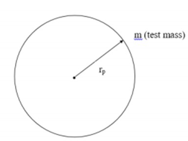
Now according to newtownian gravitation this is what we have:
our unit mass will be of size so it dissapears here.
if we wanted to find the force capability across the whole of that surface of that sphere, it would be the integral of the force across the area of that sphere.
Substituting in the equations for area of a circle and force.
I’m switching from to just for convenience.
Before we go on, there’s more stuff we have to cover. There is a theorem called the divergence theorem. You can look it up there.
Divergence: the inner product of the operator and a given vector, which gives a measure of the quantity of flux emanating from any point of the vector field or the rate of loss of mass, heat, etc., from it. - mathematics definition from google.
It says that the integral of over an area is equal to the integral over the volume of .
What that means in normal terms is that the outward flux through the area of a sphere is equal to the volume integral of the divergence of the force.
Flux describes the quantity which passes through a surface or substance.
Also I’m just going to quickly remind you that density is mass divided by volume. circa like, Archimedes probably.
In addition of course that means that the mass of an object will be an integral of the density with respect to the volume.
So then, we’ve calculated and we’ve got an equation for M as well. So let’s patch it up.
we replace M with for our definition of
Now the terms “cancel” out.
What we’re left with is
So then let’s break this down.
So far we have shown :
and remember earlier we showed that the time component of the metric tensor is equal to plus some constant leftover from that christoffel term.
and lastly that is
which means that once we put these together we get to:
the constant term dissapears here because we’ve taken a derivative.
then we find that :
The only problem is that this isn’t a tensor equation! we’re supposed to have s and s in there somewhere!
almost fun fact: is sometimes called the Einstein tensor, .
So intead of ideally we’d want some tensor to represent energy as well as pressure / density.
So we’d need to come up with a as well as something with a tensor as well.
So there’s a definition for something called a momentum 4 vector, in which we have 3 components of space and 1 vector of time.
note that here is again the proper time, and is mass. corresponds to the time dimension.
Saving myself some time here because this is the longest and most painful blog post to write, ever, you can reduce these and see what physical components they correspond to.
So this vector resolves to basic rest mass energy, plus the momentum vectors in the 3 coordinates of physical space.
But what we want here isn’t a vector , but a tensor . This actually finds itself in the form of a matrix.
| | | | | | | | | | | | | | | | | | | |
What we’re seeing is a relationship between the vectors based on the different values of and that will isolate different aspects of space when constructing the equation.
For example is just the time component of the stress energy momentum tensor.
Here’s a good diagram that shows how the tensor contains information about various different aspects of spacetime.

It is sort of like units of Energy per unit volume.
So there we are! that’s how we arrive at keeping our units consistent throughout this whole thing.
so now we have our mass term on the right hand side. We’ve solved our problem for T_{\mu \nu}. But what should our space time curvature term be on the left hand side?
The Cosmological Constant
Einstein thought that the ricci curvature tensor would be a good candidate to be this term.
The only problem is conservation of energy prevents this.
I swear we’re almost at the end of the blog post. Just like a physics lecture, we’re so far into the derivation that we’re barely aware of why we’re even doing this anymore.
If you were to take the derivative of the right hand side, you’d get zero. Unfortunately if you took a derivative of the ricci tensor on the left hand side it would not be zero. Meaning that this equation is physically impossible in it’s current state because energy is not conserved.
Einstein found that the derivative of the ricci tensor was the following:
note: it’s a good practice to always use covariant derivatives when doing this stuff.
So now let’s set our newly found to .
Now we can put our modified and back into our equation setup on the correct sides.
we need that for spacial reasons, it also corrects the units. Plus why not it’s relativity bro.
Einstein realized at this point that he had forgotten something. The equation only worked correctly when adding an additional tensor and scaling it by a constant. You see, at the time everyone believed that space was fixed, and was mostly unmoving. Yes the earth rotated around the sun but space on the whole didn’t really move around. That’s what people thought.
Bruh, so if the outer space isn't moving, shouldn't gravity be forcing the universe to collapse together? Obviously that shit ain't happening fam, so I'm gonna go out on a limb here and say something is preventing it.

That thing that was preventing it? Abraham Lincoln The cosmological constant.
It’s actually quite small and is usually left out. It’s typically only relevant when talking about large cosmological scales which is why you may see that it’s left out sometimes.
So he added in another metric tensor term, and scaled it by the cosmological constant, and here we are.
swag.
Putting the pieces together
Oh wait we’re done.
Resources
If you’ve made it this far thank you. I respect your desire to learn, and I’m sorry that I couldn’t write a better post to explain this. Here are some resources where you can learn more, from smarter people than myself. Lest I shout into the void a moment more.
-
The majority of the derivations were done really nicely in a good lecture by DrPhysicsA on youtube, you can find his two hour lecture on the topic here. A huge thank you to him for being the inspiration of the video and doing a majority of the derivations. It was really great for me to learn while writing it out.